
Timing the harvest buy: margin, volatility, and the drivers that matter
Timing a grain buy isn't a crystal-ball problem - it's a plumbing problem. Here's the whole thing as four documented API calls instead of two days of parsing USDA files.
If you have ever tried to time a grain buy off USDA source data, you know the real work is not the decision — it is the plumbing. AMS reports land as fixed-width text and inconsistent PDFs. NASS lives behind a different query model. FRED speaks its own dialect. Before you can even ask "is this a good week to cover?" you have burned two days writing parsers and reconciling units.
This piece treats the harvest-buy timing question the way an engineer would: as three data problems stacked on top of each other — a price series, a volatility read, and a margin calculation — plus one forecast layer that only applies to grains. Everything below maps to a documented DataCrop endpoint, so you can wire it up instead of scraping it.
Every response below is trimmed for readability, and the numbers in them are illustrative. The one place we quote real figures is the last section, and those come from the corn model's published metadata.
Timing a buy is a data problem, not a crystal ball
"When should I buy" decomposes into questions you can actually answer from data. Where is the price now versus its recent range? How jumpy has it been? What does that do to my margin at today's number? And — for corn, soybeans, and wheat only — what is a defensible forward range?
Notice what is not on that list: a single "the price will be X" call. We will come back to why.
Pull the price series
GET https://api.datacrop.dev/v1/series?commodity=corn&source=AMS&limit=5
Authorization: Bearer $DATACROP_KEY
{
"commodity": "corn",
"pagination": { "limit": 5, "offset": 0, "total": 1284, "has_more": true },
"series": [
{
"source": "AMS",
"source_ref": "2850",
"commodity_raw": "corn",
"date": "2026-07-27",
"value": 4.97,
"unit": "USD/BU",
"region": "US"
}
]
}Every row carries its own unit and source_ref, and that is not decoration. AMS mixes $/bu, $/cwt and $/ton across reports, so a row without its unit attached is a bug waiting to happen. source_ref pins you to one identifier — an AMS report slug, a FRED series id, a NASS commodity description — rather than a blend of several. Call /v1/identifiers to see what is available per commodity.
Corn, wheat, and soybean are the free tier: 365 days of series at 500 requests a day, which is enough to build and test the whole pipeline before paying anything.
Score the volatility
GET https://api.datacrop.dev/v1/procurement/signal?commodity=corn&weeks=13
Authorization: Bearer $DATACROP_KEY
{
"commodity": "corn",
"as_of": "2026-07-27",
"current_price": 4.97,
"price_unit": "USD/BU",
"data_window_weeks": 13,
"volatility": { "cv_pct": 6.4, "risk_level": "moderate", "risk_score": 42 },
"signal": { "price_vs_mean_pct": 2.1, "trend": "rising" }
}This is realized variation off the same series — a jumpy market and a quiet one produce visibly different numbers. weeks accepts 4 to 52 and defaults to 13, so you can ask whether this quarter has been calm relative to the last year.
The honest use of this endpoint is as a sizing input, not a trigger. A high risk_score tells you the range of outcomes is wide, which is an argument for covering in tranches rather than all at once. It does not tell you which direction the next print goes.
Procurement endpoints are Max tier. A key below that gets a 403 with {"error": "procurement_not_included"}.
Run the margin math
POST https://api.datacrop.dev/v1/procurement/margin
Authorization: Bearer $DATACROP_KEY

{ "commodity": "corn", "cost_per_unit": 4.10, "volume": 5000, "unit": "bu" }
{
"commodity": "corn",
"market": { "current_ams_price": 4.97, "price_date": "2026-07-27", "spread_vs_cost": 0.87 },
"margin": {
"break_even_price": 4.10,
"profit_per_unit": 0.87,
"total_profit": 4350.0,
"margin_pct": 17.5,
"above_break_even": true
}
}Leave selling_price out and it prices against the latest AMS quote for you; pass it explicitly to test a hypothetical. Add target_margin_pct and you also get break_even_at_target_margin, which is the number most procurement conversations actually turn on.
This is usually the endpoint that decides the buy — not the forecast.
Read the forecast band — and its limits
GET https://api.datacrop.dev/v1/forecasts?commodity=corn
Authorization: Bearer $DATACROP_KEY
{
"commodity": "corn",
"run_date": "2026-07-27",
"forecasts": [
{
"target_date": "2026-10-26",
"p10": 4.62,
"p50": 5.17,
"p90": 5.74,
"unit": "USD/BU",
"skill_vs_naive": -0.020
}
]
}Three things before you build UI on this.
Forecasts start at Pro. A free-tier key gets a 403 with {"error": "forecasts_not_included"} on this route.
Forecasts are grain-only. Corn, soybeans, and wheat. The data and the API cover every commodity we carry, but there is no forecast for cattle, cocoa, or coffee — and we would rather return nothing than return a number we cannot stand behind.
Use the band, not the midpoint. Every row ships with skill_vs_naive attached, which is the model scoring itself against a baseline that just carries today's price forward. We put it in the response on purpose. The next section is what it means.
Put it together
px   = get("/v1/series", commodity="corn", source="AMS", limit=5)   # free tier
sig  = get("/v1/procurement/signal", commodity="corn")              # Max
mgn  = post("/v1/procurement/margin", commodity="corn", cost_per_unit=my_cost)
band = get("/v1/forecasts", commodity="corn")                       # Pro+, grains only
Four calls, one auth header, consistent units. The judgment stays yours. The plumbing stops being yours.
Where this stops being magic
Here are the real numbers from the corn model's published metadata, trained through July 20, 2026.
On point accuracy, our P50 is a wash against a naive "price stays put" baseline. It is worse at the near horizons — about 8% worse at one week out. It is better in the middle of the curve, by roughly 3 to 5% at six to nine weeks. It is worse again at the far end, about 2% worse at thirteen weeks. Average that across the curve and you get a coin flip, which is the honest summary and the one we will keep publishing.
Two caveats on those figures, both about vintage. They are the corn model's metadata as trained through July 20, 2026 — the model retrains weekly, the numbers move every run, and the chart below was rendered from that same snapshot. On a later retrain corn's winning horizons shifted further out the curve. Treat these as a dated reading, not a current scoreboard; the live per-row skill_vs_naive is always in the response.
They also cover all thirteen horizons the model trains, and the API no longer serves all thirteen — see the note below, which is the part that actually changes what you receive.
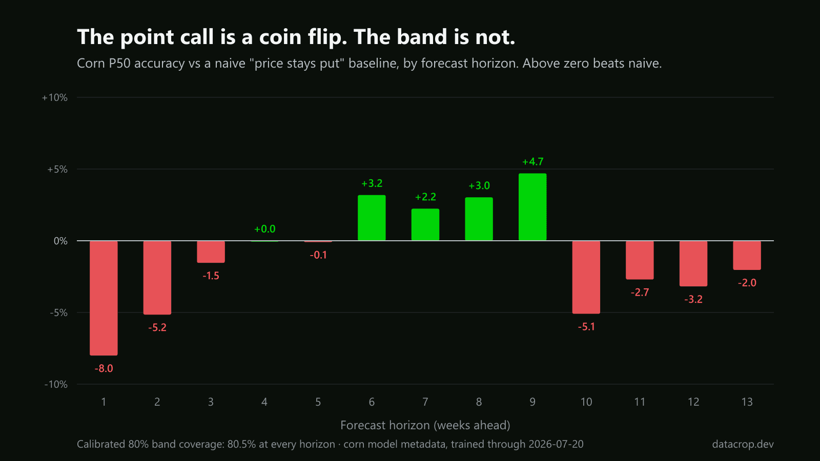
The band is calibrated *toward* 80% coverage. That is a target, not a measured hit rate, and it is worth being exact about the difference. An earlier version of this paragraph put a single number on the model's train-time holdout — the slice of history held out when the model was scored. That was itself a holdout figure presented as more settled than it is: holdout coverage isn't one flat rate, it varies by commodity and by horizon around the 80% target. Measured coverage of the bands we actually publish, scored against settled prices, currently runs below the 80% target, and we say so in the API's own method block rather than only here — as counts with their denominator, not a percentage the sample can't support.
Update, August 2026 — the forecast now runs up to three weeks, not thirteen. To be exact about why, because an earlier version of this line was not: the band did not hold its calibration to week three and then fail. Measured against the 80% target it was under at every horizon, the three we serve included, and furthest off at the long end. The cap itself came from a comparative benchmark against a band built from recent price moves on history we publish for free — a benchmark we have since had to correct (see below) — and it stands as a product decision while the corrected result is re-evaluated. The API states the cap itself, in the band_horizon_cap_note field on every response:
> The band is published to 3 weeks ahead. We capped it because we measured it, not because 3 is a round number.
Three is a ceiling, not a promise: a commodity whose data supports fewer horizons returns fewer rows.
So use the band for what a band is good for. Drop p10 and p90 into your breakeven and see which end still clears. If both ends clear, the timing question is not worth agonizing over. If only one does, you have found the actual risk in the decision, and cv_pct tells you how fast that could move.
One thing to know before you lean on it, because we would rather you heard it here. We benchmarked our band against an empirical one built purely from trailing price moves — arithmetic on the same history this endpoint serves you for free. Corrected as of August 12, 2026 (an earlier version of this paragraph said the homemade band won 133 of 143 — that count came from a benchmark whose baseline was reading post-origin prices, and it was wrong in our own favour to publish): scored across the full set of commodity-horizons, it is 100–43 in our favour raw, and 71–72 — a dead heat — once both bands are calibrated the same way. At one week out, the horizon structurally immune to that leak, the two have always been a dead heat. That benchmark, pre-correction, is what set the three-week cap quoted above — the cap stands as a product decision while the corrected result is re-evaluated — and the fuller version of the argument is in we publish our misses. Treat the band as a planning bracket, not a calibrated probability, and if you want the second thing you can build it from /v1/series yourself.
If you want the longer version of the honesty argument, we wrote it up separately in we publish our misses, and a worked post-mortem on a real move in the wheat retrospective.
Full endpoint reference, auth, rate limits and error codes are in the docs. Corn is free — you can have the first three calls working before you decide whether the fourth is worth paying for.